How to find acceleration from a position vs. time graph?
Answer: in one word, the shape of the graph shows the acceleration. A straight line means zero acceleration. A curved line means non-zero acceleration. The steeper the curve, the bigger the acceleration. A bowl shape means positive acceleration (speeding up). An upside-down bowl means negative acceleration (slowing down).
In this article, you will learn how to find the acceleration from the position-time graph, both graphically and numerically, with some solved problems for grade 12 or college level.
You can skip this introduction and refer to the worked examples.
Types of Motion:
An object can move at a constant speed or have a changing velocity.
Suppose you are driving a car at a constant speed of $100\,{\rm km/h}$ along a straight line. What does $100\,{\rm km/h}$ mean?
The speed of $100\,{\rm km/h}$ means that you drive 100 km in the first hour, another 100 km in the second hour, and so on.
If we plot these successive equal displacements as a function of time, we get a straight line.
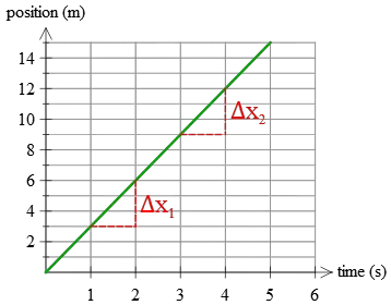
As you can see above, at equal time intervals (here, 1 second) the displacements $\Delta x_1$ and $\Delta x_2$ are equal every second.
In this type of motion, the displacements are equal during each equal time interval. This kind of motion is called uniform motion, as we learned from the average acceleration examples because the object's acceleration is zero.
From the average velocity problems, we know that $\bar{v}=\frac{x-x_0}{\Delta t}$, so we can find the position of a moving object at any instant by rearranging it as follows: \[x=vt+x_0\] This is a linear equation with a position vs. time graph shown above.
Therefore, a motion in which equal displacements occur during any successive equal-time intervals is known as uniform motion.
Now, when the car has a changing velocity, and we plot the positions of each point that the car passes through, we get a curved line, unlike the straight line in the previous case.
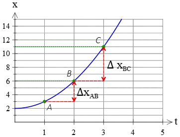
In the above, you can see explicitly that at each equal time interval (here, $1\,{\rm s}$) the corresponding displacements are not equal i.e. $\Delta x_{BC}\ne \Delta x_{AB}$.
Therefore, the acceleration of such a motion is not zero.
In this case, the position of a moving object at any moment is given by the kinematics equation, $x=\frac 12 at^2 +v_0t+x_0$. (Recall from the kinematics practice problems that this equation is for a motion with constant acceleration).
This equation tells us that for an accelerated motion, position varies with time in a quadratic form whose graph is shown above.
Overall, a constant velocity (uniform) motion has a straight-line position-versus-time graph, but a curved position-time graph represents an accelerated motion.
This curve for a constant acceleration has a simple form of a quadratic.
The direction of acceleration on a position-time graph
According to the vector definition in physics, acceleration is a vector quantity that has both a direction and a magnitude. We can find both using a position-time graph, which plots the position of an object relative to its starting point on the y-axis and the time elapsed on the x-axis.
As mentioned above, the position of a uniformly accelerating object changes with time as a quadratic function.
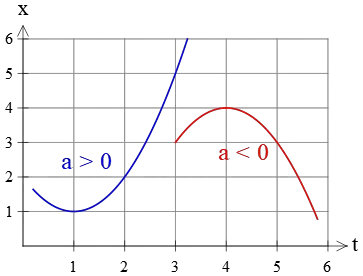
A positive acceleration ($a>0$) results in a position-time graph that curves upward.
Similarly, a negative acceleration ($a<0$) produces a position-time graph opening downward. Both cases are shown in the figure below
The magnitude of acceleration on a position-time graph
Finding the magnitude of the acceleration vector for a moving object from its position-time graph can be challenging.
If the object changes its speed at a constant rate, then its acceleration is a constant value for that time interval.
In these cases, the position vs. time graph has a quadratic shape, and we can easily find its acceleration by knowing the initial position and velocity.
In the following, we will try to learn this calculation by a couple of solved examples.
Worked Examples
Example (1): The equation of position vs. time for a moving object, in SI units, is as $x=-t^2+6t-9$. Which of the following choices is correct?
(a) The object's acceleration is constant, and its magnitude is $1\,{\rm m/s^2}$.
(b) The object's velocity at the initial time $t=0$ is to the negative $x$-axis.
(c) The object's initial position is on the negative side of the $x$-axis.
Solution: We examine each choice separately.
(a) This equation has a quadratic form, so its acceleration is constant. Comparing this equation with the standard constant acceleration kinematic equation, $x=\frac 12 at^2+v_0t+x_0$, we will find its magnitude as \[\frac 12 a=-1 \Rightarrow \ a=-2\,{\rm m/s^2}\] So this choice is incorrect.
(b) "Object's velocity at the initial time'' means its initial velocity. Comparing the two equations below reveals that the initial velocity is $v_0=+6\,{\rm m/s}$.\begin{gather*}x=\frac 12 at^2+v_0t+x_0 \\\\ x=-t^2+6t-9 \end{gather*} The positive sign indicates that the initial velocity is toward the positive $x$-axis. So, this choice is also incorrect.
(c) By setting $t=0$ in the position-time equation, its initial position is obtained. So, $x_0=-9\,{\rm m}$. Negative indicates that the object is on the negative side of the $x$-axis initially. Thus, this choice is correct.
Example (2): The position vs. time graph of a moving object that accelerates uniformly along the $x$ axis is plotted in the figure below. Find its acceleration, initial velocity, and position.
Solution: This is a positive acceleration graph because the concavity of the graph tells us about the sign of acceleration. Here, the graph opens upward (concave upward), so its acceleration is positive, $a>0$.
At the instant the motion is started $t=0$, the position of the object is a negative value. It means that, initially, the object starts its motion on the negative side of the $x$-axis.
Recall that the slope of the position-time graph represents the object's velocity. A tangent line at time $t=0$ has a negative slope because that makes an obtuse angle with the $+x$-axis. So, the initial velocity is negative, too.
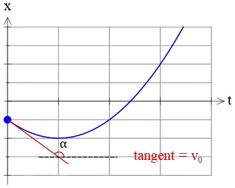
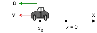
Overall, this object starts its motion at a position behind the origin in the opposite direction of the $x$-axis as shown in the figure below.
In the next example, we will find the constant acceleration of a moving object using its position vs. time graph numerically.
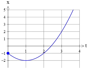
Example (3): The position of a moving object (along a straight positive line) as a function of time is given by the curve shown in the figure below. Find the acceleration of the object.
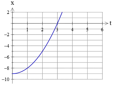
Solution: First, collect all the information that the plot gives us. At the time $t=0$, the object is in position $x=-9\,{\rm m}$, and at time $t=3\,{\rm s}$ its position is zero, that is, it returns to its starting position.
The graph opens upward, indicating a positive acceleration.
It is said that the motion has a constant acceleration, so its position versus time must be changed as a quadratic function, which is determined by the kinematics equation $x=\frac 12 at^2+v_0t+x_0$.
In the above equation, $x_0$ is the position at time $t=0$ or the initial position. The graph shows us that, for this object, it is $x_0=-9\,{\rm m}$.
$v_0$ is also the initial velocity, which is found by computing the slope of the position-time graph at time $t=0$.
As you can see, in this graph, the slope (in green) is parallel to the horizontal, making an angle of zero, and consequently, its initial velocity is zero, $v_0=0$.
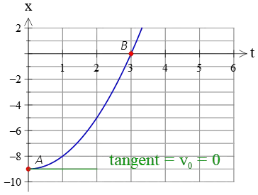
If we substitute these two findings into the standard kinematics equation $x=\frac 12 at^2+v_0t+x_0$, we get \[x=\frac 12 at^2-9\] The remaining quantity is the acceleration $a$.
There is another point that has not been used yet, $B=(x=0,t=3\,{\rm s})$. Substituting this point into the above equation, and solving for $a$ we get \begin{align*} x&=\frac 12 at^2-9\\\\0&=\frac 12 (a)(3)^2-9\\\\\Rightarrow a&=2\quad {\rm m/s^2}\end{align*} Therefore, the object's acceleration is $2\,{\rm m/s^2}$.
Example (4): A car starts at rest and accelerates at a constant rate in a straight line. Its position-versus-time graph is shown in the figure below. Find the car's acceleration.
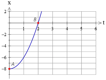
Solution: This is another example problem that shows you how to find acceleration from a position vs. time graph.
Like the previous example, locate two points on the graph with the given information. $A(x=-8\,{\rm m},t=0)$ and $B(x=0,t=2\,{\rm s})$. Using these two points and applying the kinematics equation $x=\frac 12 at^2+v_0t+x_0$, one can find the car's acceleration.
Putting point $A$ into the above equation gives us \begin{align*} x&=\frac 12 at^2+v_0t+x_0\\\\-8&=\frac 12 a(0)^2+v_0(0)+x_0\\\\\Rightarrow \quad x_0&=-8\,{\rm m}\end{align*} It is said in the question that the car starts its motion from rest, so its initial velocity is zero, $v_0=0$.
Now, substituting the second point $B$ into the standard equation, and solving for $a$, get \begin{align*}x&=\frac 12 at^2+v_0t+x_0\\\\0&=\frac 12 a(2)^2+0-8\\\\ 0&=2a-8\\\\\Rightarrow a&=4\quad {\rm m/s^2}\end{align*} So with the help of two points on the position vs. time graph, we were able to find the acceleration of the object.
In the next example, acceleration on a position-time graph is given in the case of knowing an initial velocity, $v_0\neq0$.
Example (6): The position vs. time graph of a moving object along the positive $x$-axis is as follows. Find the object's acceleration.
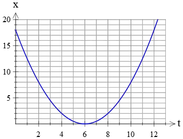
Solution: As always, to find the constant acceleration of a moving object from its position-versus-time graph, one should locate two points on the graph and substitute them into the standard kinematics equation $x=\frac 12 at^2+v_0t+x_0$.
Here, the initial point has coordinates $A(x=18\,{\rm m},t=0)$ from which we can find the initial position, $x_0=18\,{\rm m}$.
The other point is $B(x=0,t=6\,{\rm s})$. Given the initial position, substitute point B into the standard kinematics equation, and we have \begin{gather*} x=\frac 12 at^2+v_0t+x_0\\\\0=\frac 12 a(6)^2+v_0 (6)+18 \\\\ \Rightarrow \boxed{18a+6v_0+18=0} \end{gather*} As you can see, we have one equation with two unknowns. We need an additional equation to be able to find the unknowns.
In the previous examples, the position-time graph had a zero slope, so we get a zero initial velocity.
In the graph, we see that the slope at time $t=0$ is not zero, so the object does not start from rest.
But how to find another equation?
To find that equation, we pay attention to an important note below:
The tangent line at point $B$ is horizontal, so velocity at that time is zero, according to the equivalence of slope and velocity on a $x-t$ graph.
Substituting this extra information into another kinematics equation, $v=v_0+at$, we can find the initial velocity. \begin{gather*} v=v_0+at\\0=v_0+a(6)\\ \Rightarrow \boxed{6a+v_0=0} \end{gather*} Solving the above equation for $v_0$, we get $v_0=-6a$.
Now, substitute it into the first equation $18a+6v_0+18=0$ and solve for the unknown acceleration \begin{gather*} 18a+6v_0+18=0\\ 18a+6(-6a)+18=0\\ \Rightarrow a=1\quad {\rm m/s^2}\end{gather*} If we put this value into $v_0=-6a$, the initial velocity is also found.
Consequently, the car starts its motion toward the negative $x$ axis with an initial velocity of 6 m/s and increases its speed at a constant rate of $1\,{\rm m/s^2}$.
Example (7): The position vs. time graph of a moving object along a straight line is a parabola as below. Find the equation of the object's velocity as a function of time.
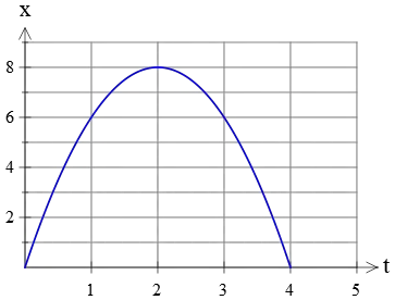
Solution: Physical interpretation of graph: This object starts its motion at some initial velocity (because the slope at time $t=0$ makes an angle with horizontal) and decreases its speed at a constant rate (i.e., $a<0$ as can be seen from the concavity downward of the curve) until it reaches point B (figure below), where its velocity gets zero, it changes its direction, and returns to the starting point in the opposite direction.
As you might guess, this is exactly the description of motion that appears in all freely falling problems. In addition, such a graph appears also in the projectile motion problems.
As said, the curve of the position-time graph is a parabola that has a quadratic form. So, the object has a constant acceleration.
On the other side, the curve opens downward, so the acceleration is negative $a<0$. In other words, such curves illustrate negative acceleration on a position vs. time graph.
In this curve, the coordinates of three points are given, $A(x=0,t=0)$, $B(x=8\,{\rm m},t=2\,{\rm s})$, and $C(x=0\,{\rm m}, t=4\,{\rm s})$.
The velocity of an object with constant acceleration changes with time as $v=v_0+at$. Thus, we must find both its initial velocity and acceleration.
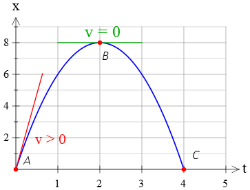
To find the unknowns, it is better to apply kinematics equations between any two given points. Between points A and B, displacement is computed as \[\Delta x=x_B-x_A=8-0=8\quad{\rm m}\] Using the kinematics equation, $v^2-v_0^2=2a\Delta x$, for these two points, we have \begin{gather*} v_B^2-v_A^2=2a\Delta x\\\\0-v_0^2=2(a)(8)\\\\\Rightarrow\quad \boxed{v_0^2=-16a}\end{gather*} where we have used this note that velocity at point B is zero because the slope of the tangent line at that point is horizontal.
Now, we choose points A and C, compute their displacement, and apply the kinematics equation $x-x_0=\frac 12 at^2+v_0t$ \[\Delta x=x_C-x_A=0-0=0\] As expected since the object returned to its starting point. \begin{gather*} \Delta x=\frac 12 at^2+v_0t\\\\0=\frac 12 (a)(4)^2+v_0(4)\\\\ \Rightarrow \quad \boxed{8a+4v_0=0} \end{gather*} Until now, we have had two equations with two unknowns that are completely solvable.
The second equation, $8a+4v_0=0$, gives us $v_0=-2a$. Now, substitute it into the first equation \begin{gather*} v_0^2=-16a\\\\ (-2a)^2=-16a\\\\4a^2=-16a\\\\ \rightarrow\quad 4a(a+4)=0\end{gather*} Solving this equation for $a$, we get two solutions $a=0$, and $a=-4\,{\rm m/s^2}$.
The zero acceleration $a=0$ is not plausible, since it represents a constant velocity motion whose position-time graph is a straight line, but in this problem, we have a curve.
Therefore, the acceptable acceleration is $a=-4\,{\rm m/s^2}$. By substituting this into either first ($v_0^2=-16a$) or second equation ($8a+4v_0$), and solving for $v_0$, we will get the initial velocity, \begin{gather*} 8a+4v_0=0 \\ \rightarrow (8)(-4)+4v_0=0\\ \Rightarrow v_0=8\,{\rm m/s}\end{gather*} As expected, since the tangent line at time $t=0$ has a positive slope.
Substituting these known values into the kinematics equation $v=v_0+at$, we will obtain the object's velocity as a function of time. \[v=8-4t\] This equation gives the variation of velocity as a function of time. When this equation is plotted, a velocity-time graph is obtained.
Summary:
In this article, we found out how to calculate the constant acceleration of an object from a position-time graph.
To do this, we need to know the initial velocity $v_0$, and the displacement $\Delta x$ between two known points on the graph. Then, we can use the kinematics equation $\Delta x=\frac 12 at^2+v_0t$ to solve for the acceleration $a$.
If the object has a non-zero initial velocity, we need at least three points on the graph with known position and time coordinates.
In this case, we can also use the kinematics equation $v^2-v_0^2=2a\Delta x$ to find the acceleration.
Author: Dr. Ali Nemati
Page Published: 8-13-2021
 kinematic
 Electrostatic
 Magnetism